Better call Thomas – Bayes in the Database

This is my third and last post covering my presentations from last week’s Tech Event, and it’s no doubt the craziest one :-).
Again I had the honour to be invited by my colleague Ludovico Caldara to participate in the cool “Oracle Database Lightning Talks” session. Now, there is a connection to Oracle here, but mainly, as you’ll see, it’s about a Reverend in a Casino.

So, imagine one of your customers calls you. They are going to use Oracle Transparent Data Encryption (TDE) in their main production OLTP database. They are in a bit of panic. Will performance get worse? Much worse?

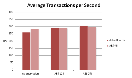
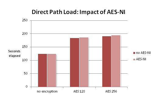
Well, you can help. You perform tests using Swingbench Order Entry benchmark, and soon you can assure them: No problem. The below chart shows average response times for one of the transaction types of Order Entry, using either no encryption or TDE with one of AES-128 or AES-256.
Wait a moment – doesn’t it even look as though response times are even lower with TDE!?

Well, they might be, or they might not be … the Swingbench results include how often a transaction was performed, and the standard deviation … so how about we ask somebody who knows something about statistics?

Cool, but … as you can see, for example, in this xkcd comic, there is no such thing as an average statistician … In short, there’s frequentist statistics and there’s Bayesian, and while there is a whole lot you can say about the respective philosophical backgrounds it mainly boils down to one thing: Bayesians take into account not just the actual data – the sample – but also the prior probability.

This is where the Reverend enters the game . The fundament of Bayesian statistics is Bayes theorem, named after Reverend Thomas Bayes.

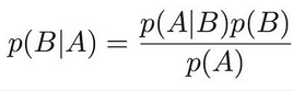
In short, Bayes Theorem says that the probability of a hypothesis, given my measured data (POSTERIOR), is equal to the the probability of the data, given the hypothesis is correct (LIKELIHOOD), times the prior probability of the hypothesis (PRIOR), divided by the overall probability of the data (EVIDENCE). (The evidence may be neglected if we’re interested in proportionality only, not equality.)

So … why should we care? Well, from what we know how TDE works, it cannot possibly make things faster! In the best case, we’re servicing all requests from the buffer cache and so, do not have to decrypt the data. Then we shouldn’t incur any performance loss. But I cannot imagine how TDE could cause a performance boost.

So we go to our colleague the Bayesian statistian, give him our data and tell him about our prior beliefs.(Prior belief sounds subjective? It is, but prior assumptions are out in the open, to be questioned, discussed and justified.).

Now harmless as Bayes theorem looks, in practice it may be difficult to compute the posterior probability. Fortunately, there is a solution:Markov Chain Monte Carlo (MCMC). MCMC is a method to obtain the parameters of the posterior distribution not by calculating them directly, but by sampling, performing a random walk along the posterior distribution.

We assume our data is gamma distributed, the gamma distribution generally being adequate for response time data (for motivation and background, see chapter 3.5 of Analyzing Computer System Performance with Perl::PDQ by Neil Gunther).
Using R, JAGS (Just Another Gibbs Sampler), and rjags, we (oh, our colleague the statistian I meant, of course) go to work and create a model for the likelihood and the prior.
We have two groups, TDE and “no encryption”. For both, we define a gamma likelihood function, each having its own shape and rate parameters. (Shape and rate parameters can easily be calculated from mean and standard deviation.)

model {
    for ( i in 1:Ntotal ) {
      y[i] ~ dgamma( sh[x[i]] , ra[x[i]] )
    }
    sh[1] <- pow(m[1],2) / pow(sd[1],2)
    sh[2] <- pow(m[2],2) / pow(sd[2],2)
    ra[1]  <- m[1] / pow(sd[1],2)
    ra[2]  <- m[2] / pow(sd[2],2
    [...]

Second, we define prior distributions on the means and standard deviations of the likelihood functions:

    [...]
    m[1] ~ dgamma(priorSha1, priorRa1)
    m[2] ~ dgamma(priorSha2, priorRa2)
    sd[1] ~ dunif(0,100)
    sd[2] ~ dunif(0,100)
  }

As we are convinced that TDE cannot possibly make it run faster, we assume that the means of both likelihood functions are distributed according to prior distributions with the same mean. This mean is calculated from the data, averaging over all response times from both groups. As a consequence, in the above code, priorSha1 = priorSha2 and priorRa1 = priorRa2. On the other hand, we have no prior assumptions about the likelihood functions’ deviations, so we model them as uniformly distributed, choosing noninformative priors.

Now we start our sampler. Faites vos jeux … rien ne va plus … and what do we get?

Here we see the outcome of our random walks, the posterior distributions of means for the two conditions. Clearly, the modes are different. But what to conclude? The means of the two data sets were different too, right?

What we need to look at is the distribution of the difference of both parameters. What we see here is that the 95% highest density interval (HDI) [3] of the posterior distribution of the difference ranges from -0.69 to +1.89, and thus, includes 0. (HDI is a concept similar, but superior to the classical frequentist confidence interval, as it is composed of the 95% values with the highest probability.)

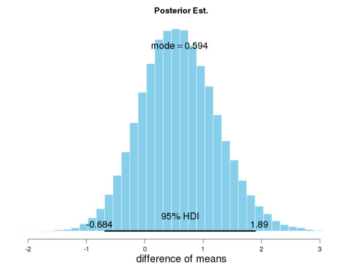
From this we conclude that statistically, our observed difference of means is not significant – what a shame. Wouldn’t it have been nice if we could speed up our app using TDE 😉

Tune the App, Not the SQL – DBA Sherlock’s Adventures in Hibernate/jOOQ Land

Last weekend at Trivadis Tech Event, in addition to my session on Oracle 12c Client High Availability for Java (Application Continuity, Transaction Guard … choose your degrees of freedom”), I gave a quite different talk called Tune the App, Not the SQL – DBA Sherlock’s Adventures in Hibernate/jOOQ Land”.

In a nutshell, what is it all about? Well, if you’re a DBA, you might sometimes (or often, or seldom – depends on your job ;-)) do what we call “SQL Tuning”. It might look like this: You get a call that the application “is slow”. Fortunately, you’re able to narrow that down quickly, and it’s just “the click on that button” that is slow. Fortunately, too, the application is well instrumented, and getting traces for specific tasks is not a problem. So you get a SQL trace file, run tkprof on it, and obtain the problematic SQLs in order of elapsed time. Then you analyse the “Top SQL”. You may find it should be rewritten, or that it would benefit from an index. Perhaps adding additional data structures might help, such as creating a materialized view. Perhaps you’re unlucky and just an ugly hint will fix it.

So you tell the developers “please rewrite that, like this”, or you create that index. And after, it’s waiting and hoping that performance will improve – noticeably, that is. Because tuning that single statement might – if you’re unlucky – not make that much of a difference.

There is, however, another approach to tuning application performance (always talking about the DB related part of it here, of course), and that has to do with the application logic and not single statements. There is an excellent demonstration of this in Stéphane Faroults very recommendable book “Refactoring SQL applications”, in fact, this is right at the beginning of the book and something that immediately “draws you in” (it was like that for me :-)).

Application logic affects what, when, and how much data is fetched. Of course, there are many aspects to this – for example, it just may not be possible to replace two DB calls by one simply because another service has to be queried in between. Also, there will have to be a tradeoff between performance and readability/maintainability of the code. But often there will be a choice. And you will see in the presentation it is not always that combining two queries into one results in better performance.

In fact, it all depends. So the first conclusion is the ubiquitous “don’t just assume, but test”.

There is another aspect to this, though. While Stéphane Faroult, in his test case, uses plain JDBC, I am using – and comparing, in a way – two commonly used frameworks: Hibernate and jOOQ. (For an “interdisciplinary introduction” to Hibernate, see my talk from previous Tech Event, Object Relational Mapping Tools – let’s talk to each other!. Quite a contrast, jOOQ is a lightweight, elegant wrapper framework providing type safety and near-100% control over the generated SQL.)

Now while for a DBA looking at a raw trace file, it will always be a challenge to “reverse engineer” application logic from the SQL sent to the database (even if plain JDBC or jOOQ are being used), the difficulties rise to a new dimension with Hibernate :-). In the talk, I am showing a DBA – who doesn’t need to be convinced any more about the importance of application logic – trying to make sense of the flow of statements in a trace file: the only information he’s got. And it turns out to be very difficult …

But as he’s not just “some DBA”, but Sherlock, he of course has his informants and doesn’t remain stuck with his DB-only view of the world – which brings me to one of my ceterum censeo’s, which is “DBAs and developers, let’s talk to each other” :-).

The slides are here.

Overhead of TDE tablespace encryption, is there?

Recently, for a customer, I conducted performance tests comparing performance under TDE tablespace encryption to a baseline. While I won’t present the results of those tests here I will describe two test series I ran in my lab environment.
So you’re an application owner – or a cautious DBA who wants to avoid trouble 😉 – and you want to know, is there an overhead if you use TDE tablespace encryption? (I think there’s some material available on this and I think it rather goes in the “no difference” direction. But it’s always nice to test for yourself, and you really need an answer – yes or no? ;-)).

For both test series, the design was the same: 2*3-factorial with factors

• encryption: none, AES 128, AES 256, and
• absence/presence of AES-NI kernel module (on suitable hardware)

So let’s see…

No there’s not!

The first test series were runs of the widely used Swingbench Order Entry Benchmark.
Measurement duration (excluding warm-up) per condition was 20 minutes, which was enough – in this isolated environment – to get reproducible results (as confirmed by sample).
The setup and environmental characteristics were the following:

• Oracle 12.1.0.2 on OEL 7
• Order Entry schema size 6G
• SGA 3G
• 2 (v)CPUs
• Data files on ASM
• 4 concurrent users

Let’s look at the results:

At first, it even looks like test runs using encryption had higher throughput. However, with standard deviations ranging between 25 and 30, for the single Order Entry transaction types, this must be attributed to chance. (Also, it would be quite difficult to argue why throughput would actually increase with TDE… let alone be highest when using an algorithm that requires more rounds of encryption…)
So from this test series, we would conclude that their is no performance impact of TDE tablespace encryption. But then, most of the time, at this ratio of schema size to buffer cache, blocks are mostly found in the cache:

• Logical read (blocks) per transaction: 105.9
• Physical read (blocks) per transaction: 2.6
• Buffer Hit %: 97.53

Now with TDE tablespace encryption, blocks are stored in the SGA unencrypted, which means only a process that has to get the block from disk has to perform decryption.
Encryption, on the other hand, is taken care of by database writer, and so happens in the background anyway. So in this setup, it’s not astonishing at all not to find throughput differences due to absence/presence of encryption.

Yes there is…

A second type of test was run against the same database, on the same host. These were SQL Loader direct path loads of a 14G file, done serially. In this case, the server process has to read every line from disk, encrypt it, and write it to disk. This is what we see in this case:

Now suddenly we DO have a substantial impact of TDE. Loading the file and storing data to disk now takes ~1.5 times as long as without encryption. And we see – which was to be expected, too – that this increase in elapsed time is mostly due to increased cpu consumption.

By the way, now that we have such a clear effect, do we see usage of AES-NI speeding up the load? No:

This is surprising and probably something deserving further investigation, but not the topic of this post…

Conclusion

So what’s the point? Whether or not you will experience negative impact on performance will depend on your workload. No simple yes-or-no here… (but of course, no mystique either. It just means we have to phrase our questions a little bit more precisely.)

Raising the Fetch Size, Good or Bad? Memory Management in Oracle JDBC 12c

Yesterday at DOAG I presented on “Raising the Fetch Size, Good or Bad? Memory Management in Oracle JDBC 12c”.
Again I’m too lazy to write a separate post (okay, let’s phrase this positively: I don’t like to be redundant ;-)) so I’ll just say what’s not in the slides …

Firstly, it all started with a story, a story about an Oracle DBA for whom, like for most any Oracle DBA I guess, fetch size was a well-known tuning knob. Most any Oracle DBA, I think, will have read some blog post on this topic, or seen a demo showing that as we raise the fetch size, throughput goes up. In fact, sometimes you can see it going up very much!

And so in one company, there was a DBA who decided to do systematic experiments, in order to find out the optimal fetch size for the in-house application. As it turned out, the optimal value for that application lay around 80. So the DBA told the developers, it was integrated into the code, and released to pre-prod. All was fine or at least nobody said the opposite.

Then inevitably, there came the day of the production release, and all wasn’t fine any more … The application server kept crashing with out of memory errors, and they had to do an emergence release, and no-one never ever wanted to talk about this any more.
What had happened? How could a value of 80 (we’re not speaking 10000 here) have such a catastrophic effect?

So that’s for the teaser… now there’s an Oracle Whitepaper where they describe how memory management in the JDBC driver was fundamentally changed between 11g and 12c. Will it be enough to read this paper, for people who have experienced those OOM errors, to be willing to try it again?
My idea was to perform an experiment and see for myself. And that’s what the talk was about, – how I set up the experiment and what was the outcome ;-). Here are the slides.

Object Relational Mapping Tools – let’s talk to each other

Following up with the follow up of Trivadis Tech Event :-).
In addition to the five minute talk about Linux Tracing for Oracle, I presented on a quite different subject: “Object Relational Mapping Tools – let’s talk to each other”.
My original intention was to write 2 – 3 successive posts on the subject, but as always, time’s scarce and so I’ve decided to just upload the presentation, see here.

But allow me some words on the background. A database admin (though spare time coder, too ;-)), presenting on O/R Mappers? How could that be? At least then, these performance killers should really get pulled to pieces, right?
Well, no. They aren’t. Instead, my intentions have been the following:

• Explain to a DBA audience why developers might want to use them.
• Explain – to DBAs and developers both – what are probable difficulties, on a conceptual level (the infamous “Object-Relational Impedance Mismatch”)
• Explain – again on a conceptual level, but with concrete examples, and to both audiences, too – what to watch out for when fetching data (i.e., doing SELECTs as opposed to data manipulation).

“What to watch out for” – this has actually been the talk’s main purpose. (I plan to follow up with load tests / “real empirical stuff” at a later time).
And how about the “let’s talk to each other”? You may have guessed already …

Peeking into Oracle using Linux tracing tools – five tools in five minutes

Five tools in five minutes?

What’s that supposed to mean, you will be asking! Well, one week ago at Trivadis Tech Event, I had the honor of being invited to participate in the Oracle Lightning Talks session organised by my colleague Ludovico Caldara, where every topic has to be presented in five minutes (which of course makes for quite an interesting “listening experience” for the audience …).
To sort of “maximize the mismatch”, I chose to present on Linux tracing tools – not one (normally you’d need hours to explain just one) – but five, one for every minute 😉

So here’s my personal list of appetizers, you’ll find some links at the end to really get you started:

strace

So, strace, you will be thinking, that sounds a bit boring, doesn’t it? Well, perhaps, but it’s a good tool to start an investigation. Oracle has its “wait event lingo”, – but what’s going on underneath?
Here for example, we’re stracing the CKPT process, who says he’s doing a control file parallel write. With strace we can see the asynchronous IO request it issued (io_submit), the two file descriptors it was issued to, and how the process waits for completion in a blocking IO call (io_getevents):

$ strace -tt -f -e write=all -v -s 100 -p $(pgrep ora_ckpt)

So strace can be useful, but beware, it will slow down the process being traced – check out Brendan Gregg’s post “Strace Wow Much Syscall” (nice title isn’t it ;-)) listed in the appendix. Speaking of whom …

https://github.com/brendangregg/perf-tools

… Brendan Gregg has a very nice collection of scripts on github, following the unix/linux philosophy, “one tool one purpose”.
Here, for example, I’m using iolatency to get a meaningful representation of IO latencies to a voting disk on one of my VMs:

$ lsblk/dev/vdb
$ ./iolatency –d 251,16

Or check out execsnoop, which shows newly created processes on the system – just watch how clusterware is constantly monitoring itself and others …

$ ./execsnoop

Useful little scripts, you could write them yourself!
Just have a look at what’s to be discovered in …

The /proc filesystem

Its content doesn’t always come as nicely formatted as the /proc/meminfo us DBAs are used to using ;-), but it may be possible to look in the kernel source to figure out what it means… For example, you might look in fs/proc/stat.c to figure out this:

$ cat /proc/stat

And perhaps even more helpful, we have lots of per-process information under /proc/<pid>/.
For example, process memory mappings, like this one here of the Oracle log writer:

$ cat /proc/$(pgrep ora_lgwr)/maps

Ok. Two left, time for the big shots… Enter –

perf

Perf has many uses, but one of the most frequent probably is sampling on-cpu functions. Say I want to determine how much overhead it is setting statistics_level to all.
I‘m executing a simple two-table join, first with statistics_level set to all, and then, with statistics_level set to typical, and for both, I sample what runs on cpu using perf. The result: not much of a difference!

$ perf record -p  -o all_hj.data sleep 30
$ perf record -p  -o typ_hj.data sleep 30
$ perf diff typ_hj.data all_hj.data

Well. Oracle was doing a hash join. Now I do the same, forcing a nested loop join, what happens?

$ perf record -p  -o all_nl.data sleep 30
$ perf record -p  -o typ_nl.data sleep 30
$ perf diff typ_nl.data all_nl.data

Oracle spends 26% of the time in a vdso call, getting the current time from the operating system!

That‘s just one example of what you can do with perf, there’s numerous others – and possibly an even more amazing tool is …

systemtap

Using systemtap, I can profile user-space (here: Oracle) functions.
This all builds upon the awesome investigations of two guys, Luca Canali and Frits Hoogland, whose work you will find linked in the appendix.
So say I’d like compare two versions of a Java program, one hard parsing all the time (using plain java.sql.Statement) and another that uses bind variables (by means of java.sql.PreparedStatement). What are they doing „under the hood“, and how long do these operations take?

This is one thing I could do: get a latency histogram of the Oracle function kksParseCursor. First, the case of doing a hard parse every time: Most parses take between 128 and 512 ms.

Then we have the code using bind variables – most parses take less than 8 ms here…

Again, this is just a starting point … possibilities are endless. So to get you started, have a look at the appendix, and: enjoy!

Appendix: What to Read

System Tap into Oracle for Fun and Profit
Life of an Oracle I/O: Tracing Logical and Physical I/O with SystemTap
Linux strace doesn’t lie after all.
How long does a logical IO take?
strace Wow Much Syscall
perf Examples

Book Review: Oracle SQL Tricks and Workarounds

Some time ago on oracle-l, someone asked for opinions regarding this book: Oracle SQL Tricks and Workarounds, by Zahar Hilkevich. As far as I know, no one knew the book (or felt like answering), and as I tend to think I know about the “books to read” in Oracle domains I’m interested in, I got curious. Plus, as a database administrator, I always have this bad conscience about not being fluent enough in SQL (What way round did it work again, connect by? How was the syntax for first_value again? … And I’m still grateful to another book – Advanced Oracle SQL Programming by Laurent Schneider – where I picked up such useful stuff as sys.odcivarchar2list…).
So I thought, I might as well get the book and write a review.

Unfortunately for me, as I do not like to criticize other people, this review will not be positive, and I was quite unsure should I really do it. Now that you read this, it’s clear how I decided, and that was for two reasons:
First, to offer people my opinion in case they’d like some buying advice, and second, more importantly, because what I think is not good about the book can be best illustrated by explaining how other approaches are better, and why, and how they do it, – which is probably the most interesting point here.

Now let me start with something positive: I do like the (intended) focus on creativity. (The question is, does the author’s method indeed result in more creative work).
Jumping right in, then, the first chapter is called “Terms and Definitions”, and here already things get strange – to put it politely. One terminological thing that bothers me may be a subjective reaction, possibly even related to my not being a native English or American speaker. The author explains how he had to choose a name for “the set of alternative solutions to a specific problem” and decided

“We call the family of distinct solutions for a given problem the workarounds for that problem.”

To me, workaround implies the existence of an obstacle, something I’ve had to work around… but well, this does not really matter, it is just a terminology thing.

Now the author has to come up with a criterion of what makes for a distinct solution, and here the decision does matter: Astonishingly, he chooses the execution plan (the plan hash value, to be precise):

“When we come up with a candidate solution, we examine its execution plan against the other solutions found so far. If it is different, we consider what we have found a new, distinct workaround; otherwise, we have only found a workaround equivalent to one of the other workarounds, which we also refer to as a synonymous workaround.”

Synonymous workaround (or solution)? In other words, things mean the same because they are executed the same way? This is a severe category error and must be incredibly confusing (and frustrating!) to SQL developers who lack any optimizer-related background knowledge. Say I rewrite my query completely, and still I get the same execution plan, – really? And then I execute it on another system, where a different Oracle version is running, and the plan is totally different? What’s the difference to trial and error? Nothing, as far as this book is concerned.

Let’s say I obtain a sizeable set of phrasings for my query, how do I decide which one is the best? In the predictive, explain plan style execution plans displayed in the book, all I may consider is the cost – may I rely on that? But choosing among different plans is not addressed by the author (guess I just execute and time the queries in my development environment ;-)). All that is addressed is how to enlarge my set of equivalent formulations.

Now, had the author just been content with showing different ways of writing SQL queries, not mixing in execution plans and pseudo-theoretic jargon, all would have been better or at least less confusing. (I also prefer – and am used to, from the “Oracle literature” in general – a much more modest style of writing, but I will not focus on that here). But given the author does show the explain plan for (just about) every rephrasing, at least he should have made some global comments about how these plans differ in general. But in the book, plans where a scan of some table is executed for every row of another table are not treated any different from plans where every table is scanned once – no ranking of plans, no comment, no nothing.

So we’re back to where I started, the “approach thing”. In a nutshell what this book does wrong is, in my opinion, to promote some sort of mechanical creativity while not providing insight. How do I get a query to run faster? I better start off with a lot of knowledge: How Oracle works, how the query optimizer works, what Oracle does with the query I’m passing in, how queries get transformed and why, how access paths are chosen and why… This is one kind of story (next to, e.g., the reverse engineering adventures) I always love reading on Jonathan Lewis’ blog: He knows what kind of execution plan, what access paths etc. he wants and then he rewrites and/or hints the query until he is there :-).

So optimizer and performance related knowledge is key, and for that, I totally recommend studying another book: Chris Antognini’s Troubleshooting Oracle Performance. Most readers will surely know the book, so I won’t add much more here, apart from it definitely being one of my “Oracle books to take on a lone island” if I were to choose 😉

Secondly, as we’re not talking about Oracle Performance in general, but SQL performance specifically, it certainly makes sense to work on specific techniques and methods (like analytic functions, set-based thinking, model clause etc) – and in general, to keep up with what’s going on, sql-wise, as new Oracle versions get out. In this domain, one book I liked and found instructive was Pro Oracle SQL.

Thirdly, a methodological approach may work, if it is based on criteria that really play a role in execution plans. Although I have no personal experience with it, it may be interesting to look into SQL Tuning, by Dan Tow, who bases his methods on relevant (single-table and join) selectivities.

Of course, this book list is not exhaustive, – the main point is, we have some wonderful, insight-providing books around in the Oracle Performance domain, there’s no need for trial-and-error if we want to be creative :-).

Bind variables vs. literals, a quiz and a surprise

The quiz

Recently, something I had intended to be a simple demo promoting the use of bind variables among Java developers turned out to be more interesting than expected.
It all started as a quiz. So I was going to ask, how long would the following run:

• a fixed query, repeated 100,000 times, always with the same literal
• the same query, again repeated 100,000 times, but this time using a bind variable, the same value every time
• the same query, repeated 100,000 times, using 100,000 different literals
• the same query, repeated 100,000 times, using 100,000 different values for the bind variable

Just so you know what I did exactly, this is how the Java code looked (displaying the relevant parts here only):

One same literal, 100,000 times

String query = "select text1, text2 from mytab where rn=";
int id = 1;
long startTime = System.currentTimeMillis();
Statement stmt = conn.createStatement();
for (int i = 0; i <= 100000; i++) {
  ResultSet rset = stmt.executeQuery (query + id);
  String s;
  while (rset.next ()) {
    s = rset.getString (1) + " " + rset.getString (2);
  }
  rset.close();
}
stmt.close();
System.out.println(System.currentTimeMillis() - startTime);
conn.close();

One same bind value, 100,000 times

String query = "select text1, text2 from mytab where rn=?";
int id = 1;
long startTime = System.currentTimeMillis();
PreparedStatement stmt = conn.prepareStatement(query);
for (int i=0; i<= 100000; i++) {
  stmt.setInt(1, id);
  ResultSet rset = stmt.executeQuery();
  String s;
  while (rset.next ()) {
    s = rset.getString (1) + " " + rset.getString (2);
  }
  rset.close();
}
stmt.close();
System.out.println(System.currentTimeMillis() - startTime);
conn.close();

100,000 different literals

String query = "select text1, text2 from mytab where rn=";
int id = 1;
long startTime = System.currentTimeMillis();
Statement stmt = conn.createStatement();
for (int i = 0; i<= 100000; i++) {
  ResultSet rset = stmt.executeQuery (query + id);
  String s;
  while (rset.next ()) {
    s = rset.getString (1) + " " + rset.getString (2);
  }
  rset.close();
  id = id + 1;
}
stmt.close();
System.out.println(System.currentTimeMillis() - startTime);
conn.close();

100,000 different bind values

String query = "select text1, text2 from mytab where rn=?";
int id = 1;
long startTime = System.currentTimeMillis();
PreparedStatement stmt = conn.prepareStatement(query);
for (int i = 0; i<= 100000; i++) {
  stmt.setInt(1, id);
  ResultSet rset = stmt.executeQuery();
  String s;
  while (rset.next ()) {
    s = rset.getString (1) + " " + rset.getString (2);
  }
  rset.close();
  id = id + 1;
}
stmt.close();
conn.close();

So, of course what I intended to show was the devastating effect of using different literals all the time. Which I succeeded in. But let’s look at the results, first, the execution times measured on the client side:

Client-side execution times (ms)

One same literal	36.1
One same bind value	24.7
100,000 literals	147.4
100,000 bind values	25.3

The surprise

Nice. The 100,000 different literals case does have a horrible execution time. But let’s look at the one-same-value cases, same literal vs. same bind value. Why is the bind variable case so much faster?
(And by the way, although I’m listing the results of one trial only, they were totally reproducible, the pattern was the same how ever I varied the circumstances – e.g., with/without tracing …)

In the one-same-literal case, we perform one hard parse and two soft parses, – from there on it’s “softer soft parses” only.
This can nicely be seen in the trace file. In the third CLOSE line, we have type=1, and PARSE elapsed times are <30 microseconds from there on:

PARSING IN CURSOR ...
PARSE #140263995577416:c=2999,e=20813,p=0,cr=0,cu=0,mis=1,r=0,dep=0,og=1,plh=2832086359,tim=1420822842233661
EXEC #140263995577416:c=0,e=69,p=0,cr=0,cu=0,mis=0,r=0,dep=0,og=1,plh=2832086359,tim=1420822842238446
WAIT #140263995577416: nam='SQL*Net message to client' ela= 4 driver id=1413697536 #bytes=1 p3=0 obj#=-1 tim=1420822842238488
FETCH #140263995577416:c=0,e=110,p=0,cr=4,cu=0,mis=0,r=1,dep=0,og=1,plh=2832086359,tim=1420822842238639
..
WAIT #140263995577416: nam='SQL*Net message from client' ela= 101732 driver id=1413697536 #bytes=1 p3=0 obj#=-1 tim=1420822842340650
CLOSE #140263995577416:c=0,e=15,dep=0,type=0,tim=1420822842340788
=====================
PARSING IN CURSOR ... 
PARSE #140263995577416:c=0,e=199,p=0,cr=0,cu=0,mis=0,r=0,dep=0,og=1,plh=2832086359,tim=1420822842341057
EXEC #140263995577416:c=0,e=46,p=0,cr=0,cu=0,mis=0,r=0,dep=0,og=1,plh=2832086359,tim=1420822842341161
WAIT #140263995577416: nam='SQL*Net message to client' ela= 3 driver id=1413697536 #bytes=1 p3=0 obj#=-1 tim=1420822842341197
FETCH #140263995577416:c=0,e=44,p=0,cr=4,cu=0,mis=0,r=1,dep=0,og=1,plh=2832086359,tim=1420822842341312
...
WAIT #140263995577416: nam='SQL*Net message from client' ela= 1708 driver id=1413697536 #bytes=1 p3=0 obj#=-1 tim=1420822842343128
CLOSE #140263995577416:c=0,e=8,dep=0,type=0,tim=1420822842343193
=====================
PARSING IN CURSOR ...
PARSE #140263995577416:c=0,e=52,p=0,cr=0,cu=0,mis=0,r=0,dep=0,og=1,plh=2832086359,tim=1420822842343301
EXEC #140263995577416:c=0,e=30,p=0,cr=0,cu=0,mis=0,r=0,dep=0,og=1,plh=2832086359,tim=1420822842343386
WAIT #140263995577416: nam='SQL*Net message to client' ela= 1 driver id=1413697536 #bytes=1 p3=0 obj#=-1 tim=1420822842343414
FETCH #140263995577416:c=0,e=29,p=0,cr=4,cu=0,mis=0,r=1,dep=0,og=1,plh=2832086359,tim=1420822842343467
...
WAIT #140263995577416: nam='SQL*Net message from client' ela= 1618 driver id=1413697536 #bytes=1 p3=0 obj#=-1 tim=1420822842345279
CLOSE #140263995577416:c=0,e=14,dep=0,type=1,tim=1420822842345357
PARSE #140263995577416:c=0,e=27,p=0,cr=0,cu=0,mis=0,r=0,dep=0,og=1,plh=2832086359,tim=1420822842345420
EXEC #140263995577416:c=0,e=31,p=0,cr=0,cu=0,mis=0,r=0,dep=0,og=1,plh=2832086359,tim=1420822842345473
WAIT #140263995577416: nam='SQL*Net message to client' ela= 1 driver id=1413697536 #bytes=1 p3=0 obj#=-1 tim=1420822842345502
FETCH #140263995577416:c=0,e=27,p=0,cr=4,cu=0,mis=0,r=1,dep=0,og=1,plh=2832086359,tim=1420822842345568
WAIT #140263995577416: nam='SQL*Net message from client' ela= 1618 driver id=1413697536 #bytes=1 p3=0 obj#=-1 tim=1420822842347230
CLOSE #140263995577416:c=0,e=11,dep=0,type=3,tim=1420822842347318

From a visual inspection of the trace file for the one-same-bind-value case, you might think both cases should take about the same time in the end:

PARSING IN CURSOR ...
PARSE #140450201769032:c=0,e=873,p=0,cr=0,cu=0,mis=1,r=0,dep=0,og=1,plh=0,tim=1420823096225812
EXEC #140450201769032:c=2000,e=2337,p=0,cr=0,cu=0,mis=1,r=0,dep=0,og=1,plh=2832086359,tim=1420823096228602
WAIT #140450201769032: nam='SQL*Net message to client' ela= 4 driver id=1413697536 #bytes=1 p3=0 obj#=-1 tim=1420823096228684
FETCH #140450201769032:c=0,e=112,p=0,cr=4,cu=0,mis=0,r=1,dep=0,og=1,plh=2832086359,tim=1420823096228869
...
WAIT #140450201769032: nam='SQL*Net message from client' ela= 83168 driver id=1413697536 #bytes=1 p3=0 obj#=-1 tim=1420823096312251
EXEC #140450201769032:c=0,e=71,p=0,cr=0,cu=0,mis=0,r=0,dep=0,og=1,plh=2832086359,tim=1420823096312442
WAIT #140450201769032: nam='SQL*Net message to client' ela= 2 driver id=1413697536 #bytes=1 p3=0 obj#=-1 tim=1420823096312507
FETCH #140450201769032:c=0,e=60,p=0,cr=4,cu=0,mis=0,r=1,dep=0,og=1,plh=2832086359,tim=1420823096312527
WAIT #140450201769032: nam='SQL*Net message from client' ela= 1081 driver id=1413697536 #bytes=1 p3=0 obj#=-1 tim=1420823096313684
EXEC #140450201769032:c=0,e=36,p=0,cr=0,cu=0,mis=0,r=0,dep=0,og=1,plh=2832086359,tim=1420823096313794
WAIT #140450201769032: nam='SQL*Net message to client' ela= 1 driver id=1413697536 #bytes=1 p3=0 obj#=-1 tim=1420823096313832
FETCH #140450201769032:c=0,e=35,p=0,cr=4,cu=0,mis=0,r=1,dep=0,og=1,plh=2832086359,tim=1420823096313848

How does this go together then – on the one hand, the work done by the database does not seem to be tremendously different, on the other, the bind values case is noticeably faster on the client!

Well, let’s look at a statistical summary of the database calls for both cases.
First, the one-same-literal case:

1 same literal, 100,000 times

call type	count	sum elapsed	avg elapsed	stddev elapsed	median elapsed
PARSE	100001	1850716	19	20	16
EXEC	100001	1207545	12	12	11
FETCH	100001	1384287	14	17	12
CLOSE	100000	335618	3	4	3
overall db	400003	4778166

1 same bind value, 100,000 times

call type	count	sum elapsed	avg elapsed	stddev elapsed	median elapsed
PARSE	1	202	202	0	202
EXEC	100001	1388479	14	25	12
FETCH	100001	3080674	31	30	28
CLOSE	0
overall db	200003	4469355

So it’s true, seen from the database side, the elapsed times for both cases do not differ much at all!
So really the database is doing about the same amount of work in both cases.

Wait a sec …

What about when we add the wait time, especially, SQL*NET message from client (overall db calls are the db call summary numbers from above)?

1 same literal, 100,000 times

type	count	sum elapsed	avg elapsed	stddev elapsed	median elapsed
SQL*NET msg from client	100001	15308493	153	949	106
overall db calls	400003	4778166
overall total	500004	20086659

1 same bind value, 100,000 times

type	count	sum elapsed	avg elapsed	stddev elapsed	median elapsed
SQL*NET msg from client	100001	11425310	114	416	74
overall db calls	200003	4469355
overall total	300004	15894665

So we see it is really the time subsumed under SQL*NET message from client that makes the difference.
Why? A SQL*NET trace shows that the amount of data transferred over the network is about twice as much for the literals case than for the binds case (156 vs. 70 bytes per execution). Of course, that’s way below TCP packet size in both cases, but the data has to pass various layers where the size of the read/write operations might make a difference. Probably, the biggest factor here might be the processing on the Java client side, the client having to marshal either a simple number or a not-too-short string. (Of course, that’s just a guess which would need to be supported by more sophisticated measurements on the client side.)

So what’s the conclusion? We can be even more confident about advising (Java) developers to use bind variables, because response times will go down even in cases where one (me, at least) wouldn’t have expected to see a noticeable difference 🙂

SQL trace files, think time, and outliers

Idle wait events and think time

When creating a resource profile for a session or a group of sessions, one usually has to decide how to handle the so-called idle wait events, first and foremost, SQL*Net message from client.

One possibility would be to simply remove (physically or logically) those lines from the trace, thereby avoiding the question of whether some wait should be classified as client (= application) response time, or as think time.
Another would be be to define a threshold and exclude only those lines with wait times above the threshold. In that case, of course, I have to know what makes for a sensible threshold. I could base that threshold on network latencies but then, I might miss information about how the application behaves – what, from the database server’s point of view, is the response time of the application?

So here I want to try another approach, which is applying common outlier detection methods and find out how far that gets me ;-). My test material, this time, will be “real life”, non-artificial trace files, my tools will be the mining infrastructure based on external tables described in the latest three blog posts (starting with Mining SQL Trace Files Using External Tables Part 1: Getting the Timeline and, for ease of use, uploaded on github, and the outlier detection methods used will be four common ones described in http://d-scholarship.pitt.edu/7948/1/Seo.pdf.

Outlier detection methods

The four methods chosen were selected for being both commonly used as well as easily applicable. None of them are based on hypothesis testing as this would require knowledge of the underlying distribution.

Standard deviation method

One commonly used method is classifying as outliers those measurements whose distance from the mean is more than 2 or 3 standard deviations. We may already suspect that a method based on the normality assumption might not be the most effective here, but we’ll have a look anyway, be it only for establishing a baseline for the other methods.

Boxplot

As per Tukey’s boxplot method, values are seen as outliers when either below the first quartile minus 1.5* (3*, respectively) the interquartile range or above the third quartile plus 1.5 * (3*, respectively) the interquartile range (i.e., x < Q1 – 1.5[3]*IQR or x > Q3 + 1.5[3]*IQR).

MAD_e

Using the MAD_e method, values are classified as outliers when there distance from the median is more than 2 times (3 times, respectively) the median of absolute differences from the median, scaled by 1.483 (this scaled median of absolute differences is the so-called MAD_e).
I.e., x < median – 2[3] MAD_e or x > median – 2[3] MAD_e.

Median method

Using the median method, values are classified as outliers when they are below/above the median by more than n*IQR, when n is adjustable and chosen as 2.3 in the above mentioned paper.

Outlier detection methods applied

Inspecting the data

First, for all four trace files, let me indicate some summary statistics for the SQL*Net message from client event and present the data graphically.
All trace files have about 50.000 lines for this wait event, with minimum values of ~ 0.35-0.55 milliseconds, a median value of ~ 0.55-0.75 ms, an average of ~1.5-1.8 ms and a maximum ranging from 2.2 to 12 seconds approximately.

SQL> select min(elapsed) min, median(elapsed) median, trunc(avg(elapsed)) avg, trunc(stddev(elapsed)) stddev, max(elapsed) max, count(elapsed) cnt from wait where event='SQL*Net message from client';

-- file 1
       MIN     MEDIAN	     AVG     STDDEV	   MAX	      CNT
---------- ---------- ---------- ---------- ---------- ----------
       368	  541	    1606      33961    3005346	    53124

-- file 2
       MIN     MEDIAN	     AVG     STDDEV	   MAX	      CNT
---------- ---------- ---------- ---------- ---------- ----------
       523	  683	    1843      33805    2269024	    51485

-- file 3
       MIN     MEDIAN	     AVG     STDDEV	   MAX	      CNT
---------- ---------- ---------- ---------- ---------- ----------
       339	  530	    1530      68874   11794066	    47152

-- file 4
       MIN     MEDIAN	     AVG     STDDEV	   MAX	      CNT
---------- ---------- ---------- ---------- ---------- ----------
       547	  770	    1482      27795    3306050	    52608

The following diagrams should help visualize how the data is distributed. I’ve chosen a bucket size of 250 microseconds/0.25 milliseconds, which after some experimentation seemed to work best.
(This means that the numbers on the x axis have to be multiplied by 0.25 to give the elapsed time in microseconds).

For all methods, I’m interested in the upper threshold only. Now let’s see what the different methods yield.

Standard deviation method

with sd_data as
  (select avg(elapsed) avg, stddev(elapsed) stddev from wait where event='SQL*Net message from client'),
  bounds as 
    (select avg + 2*stddev upper_2sd, avg + 3*stddev upper_3sd from sd_data),
    candidates_2sd as
      (select elapsed from wait w join bounds b on (w.event='SQL*Net message from client' and w.elapsed >  b.upper_2sd)),
      candidates_3sd as
        (select elapsed from wait w join bounds b on (w.event='SQL*Net message from client' and w.elapsed >  b.upper_3sd))
        select '   2sd' "method", count(elapsed) "num_outliers", round(min(elapsed)/1000, 1) "smallest_outlier_ms", round(max(elapsed)/1000, 1) "max_value_ms" from candidates_2sd
        union all 
        select '   3sd', count(elapsed), round(min(elapsed)/1000, 1), round(max(elapsed)/1000, 1) from candidates_3sd;


-- file 1
method num_outliers smallest_outlier_ms  max_value_ms
------ ------------ ------------------- -------------
   2sd		 64		   75.2        3005.3
   3sd		 62		  106.6        3005.3

-- file 2
method num_outliers smallest_outlier_ms max_value_ms
------ ------------ ------------------- ------------
   2sd		 88		   70.5 	2269
   3sd		 84		  116.3 	2269

-- file 3
method num_outliers smallest_outlier_ms max_value_ms
------ ------------ ------------------- ------------
   2sd		 31		  145.9      11794.1
   3sd		 26		  221.7      11794.1

-- file 4
method num_outliers smallest_outlier_ms max_value_ms
------ ------------ ------------------- ------------
   2sd		 64		   62.4       3306.1
   3sd		 55		     93       3306.1

Not surprisingly (given the non-normality of the data), the standard deviation method does not yield useful results. We’ll certainly want to classify as think time values well below 100 ms.

Boxplot

with iqr_data as 
  (select percentile_cont(0.25) within group (order by elapsed) q1, percentile_cont(0.75) within group (order by elapsed) q3, abs(percentile_cont(0.25) within group (order by elapsed) - percentile_cont(0.75) within group (order by elapsed)) iqr from wait where event='SQL*Net message from client'),
  bounds as 
    (select q3 + 1.5 * iqr lower_bound, q3 + 3 * iqr upper_bound from iqr_data),
      candidates_inner as
          (select elapsed from wait w join bounds b on (w.event='SQL*Net message from client' and w.elapsed >  b.lower_bound)),
          candidates_outer as
            (select elapsed from wait w join bounds b on (w.event='SQL*Net message from client' and w.elapsed >  b.upper_bound))
            select 'outside inner bound' "criterion", count(elapsed) "num_outliers", round(min(elapsed)/1000, 1) "smallest_outlier_ms", round(max(elapsed)/1000, 1) "max_value_ms" from candidates_inner
            union all
            select 'outside outer bound', count(elapsed), round(min(elapsed)/1000, 1), round(max(elapsed)/1000, 1) from candidates_outer
        ;
   

-- file 1
criterion	    num_outliers smallest_outlier_ms max_value_ms
------------------- ------------ ------------------- ------------
outside inner bound	    5370		  .9	   3005.3
outside outer bound	    3983		 1.1	   3005.3

-- file 2
criterion	    num_outliers smallest_outlier_ms max_value_ms
------------------- ------------ ------------------- ------------
outside inner bound	    3869		   1	     2269
outside outer bound	    2264		 1.2	     2269

-- file 3
criterion	    num_outliers smallest_outlier_ms max_value_ms
------------------- ------------ ------------------- ------------
outside inner bound	    2026		  .8	  11794.1
outside outer bound	     809		  .9	  11794.1

-- file 4
criterion	    num_outliers smallest_outlier_ms max_value_ms
------------------- ------------ ------------------- ------------
outside inner bound	    3836		 1.1	   3306.1
outside outer bound	    1418		 1.3	   3306.1

This looks better! If we choose the outer bound, waits have to exceed 1 ms to be classified as think time. However, looking at the diagrams, I’m not sure if this is not too low. Let’s compare with median-based methods.

MAD_e

with median as
  (select median(elapsed) median from wait where event='SQL*Net message from client'),
  abs_differences as
    (select abs(elapsed - median) absdiff from wait, median),
    mad_e as 
      (select median(absdiff) mad_e from abs_differences),
        bounds as 
          (select median + 2*mad_e upper_2mad_e, median + 3*mad_e upper_3mad_e from median, mad_e),
          candidates_2mad_e as
            (select elapsed from wait w join bounds b on (w.event='SQL*Net message from client' and w.elapsed >  b.upper_2mad_e)),
            candidates_3mad_e as
              (select elapsed from wait w join bounds b on (w.event='SQL*Net message from client' and w.elapsed >  b.upper_3mad_e))
                select '2mad_e' "method", count(elapsed) "num_outliers", round(min(elapsed)/1000, 1) "smallest_outlier_ms", round(max(elapsed)/1000, 1) "max_value_ms" from candidates_2mad_e
                union all 
                select '3mad_e', count(elapsed), round(min(elapsed)/1000, 1), round(max(elapsed)/1000, 1) from candidates_3mad_e;


-- file 1
method	num_outliers smallest_outlier_ms max_value_ms
------- ------------ ------------------- ------------
2mad_e   	2740		     1.6       3005.3
3mad_e  	1523		     2.2       3005.3

-- file 2
method num_outliers smallest_outlier_ms max_value_ms
------ ------------ ------------------- ------------
2mad_e		287		      2 	2269
3mad_e		208		    2.7 	2269

-- file 3
method num_outliers smallest_outlier_ms max_value_ms
------ ------------ ------------------- ------------
2mad_e		236		    1.6      11794.1
3mad_e		142		    2.1      11794.1

-- file 4
method num_outliers smallest_outlier_ms max_value_ms
------ ------------ ------------------- ------------
2mad_e		487		    2.3       3306.1
3mad_e		380		    3.1       3306.1

Now this – again choosing the outer bound, so we end up at a threshold of ~ 2-2.5 ms, looks much better to me. Perhaps it is still a little low, from visual inspection?

Median method

with iqr_data as 
  (select median(elapsed) median, percentile_cont(0.25) within group (order by elapsed) q1, percentile_cont(0.75) within group (order by elapsed) q3, abs(percentile_cont(0.25) within group (order by elapsed) - percentile_cont(0.75) within group (order by elapsed)) iqr from wait where event='SQL*Net message from client'),
  bounds as 
    (select median + 2.3 * iqr bound from iqr_data),
      candidates as
          (select elapsed from wait w join bounds b on (w.event='SQL*Net message from client' and w.elapsed >  b.bound))
            select 'outside bound' "criterion", count(elapsed) "num_outliers", round(min(elapsed)/1000, 1) "smallest_outlier_ms", round(max(elapsed)/1000, 1) "max_value_ms" from candidates;


-- file 1   
criterion     num_outliers smallest_outlier_ms max_value_ms
------------- ------------ ------------------- ------------
outside bound	      5065		    .9	     3005.3

-- file 2
criterion     num_outliers smallest_outlier_ms max_value_ms
------------- ------------ ------------------- ------------
outside bound	      3575		     1	       2269

-- file 3
criterion     num_outliers smallest_outlier_ms max_value_ms
------------- ------------ ------------------- ------------
outside bound	      1729		    .8	    11794.1

-- file 4
criterion     num_outliers smallest_outlier_ms max_value_ms
------------- ------------ ------------------- ------------
outside bound	      3316		   1.1	     3306.1

The median method, at least for the trace files given, seems to yield results very similar to boxplot. Same as with boxplot, it might be too strict though.

Conclusion

Of course, four trace files, taken from the same application and under similar conditions, do not make for a representative sample. However, the idea here was to demonstrate the approach, i.e., looking at think time from an outlier detection perspective. For the given sample, the MAD_e method seems to yield a plausible classification. However, what classification makes sense is, in the end, a question of (at least) two things – the application we’re looking at (a real application? or end users, sitting at their terminals?) and what we want to do with the data (diagnose the database only or the client, too).

I guess it’s the latter case when this approach will be the most useful.

.

Monitoring execution plan changes

Times being a bit busy for me at the moment, unfortunately I have to postpone any “larger” projects, blogging-wise 😉 … but not wanting to lose the habit, I’ve thought I’d publish a little script I’ve written to track changes in execution plans.

The intention is to alert DBAs / developers to SQL statements that due to plan changes have experienced large variation in execution time.
When run, as I’d suggest, every day, the script quickly points out statements whose elapsed time at the most recent point of measurement is much different (in either direction) from elapsed times encountered in earlier snapshots that form part of the comparison moving window.

The moving window size, as well as the threshold (what kind of difference should be considered a big difference?) are parameterized. Different environments / applications will have different optimal values here, plus you will have to find a configuration where the amount of information (number of changed plans) can be handled by the DBAs 🙂

So, here’s the script.

set sqlblanklines on
set lines 800
set pages 1000

/* statements captured during last  days */
with samples as 
 (select *
  from dba_hist_sqlstat st
  join dba_hist_snapshot sn
  using (snap_id, instance_number) 
  where parsing_schema_name = '&schema_name'
  and module  'DBMS_SCHEDULER' -- no sql tuning task
  and executions_delta > 0
  and begin_interval_time between sysdate - '&num_days' and sysdate),

/* just statements that had at least 2 different plans during that time */
  sql_ids as 
   (select sql_id,
    count(distinct plan_hash_value) plancount
    from samples
    group by sql_id
    having count(distinct plan_hash_value) > 2),

/* per combination of sql_id and plan_hash_value, elapsed times per execution */
    plan_stats as 
     (select sql_id,
      plan_hash_value,
      count(snap_id) snap_count,
      max(end_interval_time) last_seen,
      sum(executions_delta) total_execs,
      sum(elapsed_time_delta) / sum(executions_delta) elapsed_per_exec_thisplan
      from sql_ids
      join samples
      using (sql_id)
      group by sql_id, plan_hash_value),

/* how much different is the elapsed time most recently encountered from other elapsed times in the measurement interval? */
      elapsed_time_diffs as 
       (select p.*,
        elapsed_per_exec_thisplan - first_value(elapsed_per_exec_thisplan)
          over(partition by sql_id order by last_seen desc) elapsed_per_exec_diff,
        (elapsed_per_exec_thisplan - first_value(elapsed_per_exec_thisplan)
          over(partition by sql_id order by last_seen desc)) / elapsed_per_exec_thisplan elapsed_per_exec_diff_ratio
        from plan_stats p),

/* consider just statements for which the difference is bigger than our configured threshold */
        impacted_sql_ids as 
         (select *
          from elapsed_time_diffs
          where abs(elapsed_per_exec_diff_ratio) > &threshold),

/* for those statements, get all required information */
          all_info as
           (select sql_id,
            plan_hash_value,
            snap_count,
            last_seen,
            round(elapsed_per_exec_thisplan / 1e6, 2) elapsed_per_exec_thisplan,
            round(elapsed_per_exec_diff / 1e6, 2) elapsed_per_exec_diff,
            round(100 * elapsed_per_exec_diff_ratio, 2) elapsed_per_exec_diff_pct,
            round(max(abs(elapsed_per_exec_diff_ratio))
              over(partition by sql_id), 2) * 100 max_abs_diff,
            round(max(elapsed_per_exec_diff_ratio) over(partition by sql_id), 2) * 100 max_diff,
            'select * from table(dbms_xplan.display_awr(sql_id=>''' || sql_id ||
            ''', plan_hash_value=>' || plan_hash_value || '));' xplan
            from elapsed_time_diffs
            where sql_id in (select sql_id from impacted_sql_ids))

/* format the output */
            select case sign(elapsed_per_exec_diff)
              when 0 then max_abs_diff ||
                case when max_abs_diff  max_diff then
                  '% worse than another plan found during the last 7 days'
                else
                  '% better than the next best plan during the last 7 days'
                end
             end status,
             a.sql_id,
             a.snap_count,
             to_char(last_seen, 'yy-mm-dd hh24:mi:ss') last_seen,
             to_char(a.elapsed_per_exec_thisplan, '999999.99') elapsed_per_exec_thisplan,
             to_char(a.elapsed_per_exec_diff, '999999.99') elapsed_per_exec_diff,
             to_char(a.elapsed_per_exec_diff_pct, '999999.99') elapsed_per_exec_diff_pct,
             xplan
             from all_info a
             order by sql_id, last_seen desc;

And this is how it might look (“pivoting” the output to make it readable here, and showing one statement only):

status                       	9073% worse than another plan found during the last 7 days 
sql_id   			698s47bt259sk
snap_count 			5
last_seen       		14-09-22  06:30:07
elapsed_per_exec_thisplan	315.74 
elapsed_per_exec_diff 		.00
elapsed_per_exec_diff_pct  	.00
xplan       			select * from table (dbms_xplan.dislay_awr(sql_id=>'698s47bt259sk', plan_hash_value=>3533318143));
                                                                                        
sql_id   			698s47bt259sk
snap_count 			5
last_seen       		14-09-22  06:30:07
elapsed_per_exec_thisplan	3.44 
elapsed_per_exec_diff 		-312.29
elapsed_per_exec_diff_pct  	-9072.77
xplan       			select * from table (dbms_xplan.dislay_awr(sql_id=>'698s47bt259sk', plan_hash_value=>3837578073));

Of course, the script would have to be adapted if you had to deal with statements using different literals on each execution (which was not the case for my usecase this time).